Everything you need to know about model evaluation — from your first confusion matrix to evaluating AI agents — without the textbook.

Imagine you hire a weather forecaster. Every single day, they confidently say “No rain tomorrow.” You live in a desert. They’re right 340 days out of 365. Their accuracy? 93%. Are they a good forecaster?

No. They learned one trick and are riding it.

This is the core problem with evaluating AI. A number that looks great on paper can mean absolutely nothing — or be dangerously misleading — if you’re measuring the wrong thing. And in my experience, most teams are.

This post is about getting that right. We’ll go from the basics (how to split your data without lying to yourself), through every major metric you actually need to know, into the world of LLMs grading other LLMs, and all the way to the genuinely unsolved problem of evaluating AI agents. I’ll tell you when each tool applies, when it doesn’t, and which ones people consistently misuse.

One thing up front: metrics are not truth. They’re proxies. Every metric measures something specific. None of them measure “is this AI good?” in the abstract. The evaluation trap is optimizing for the metric instead of optimizing for what the metric was supposed to represent. Keep that sentence in your head for the rest of this post.

First, don’t cheat on your own test

Before you evaluate anything, you need data that the model has never seen. This sounds obvious. It’s not as obvious as it sounds.

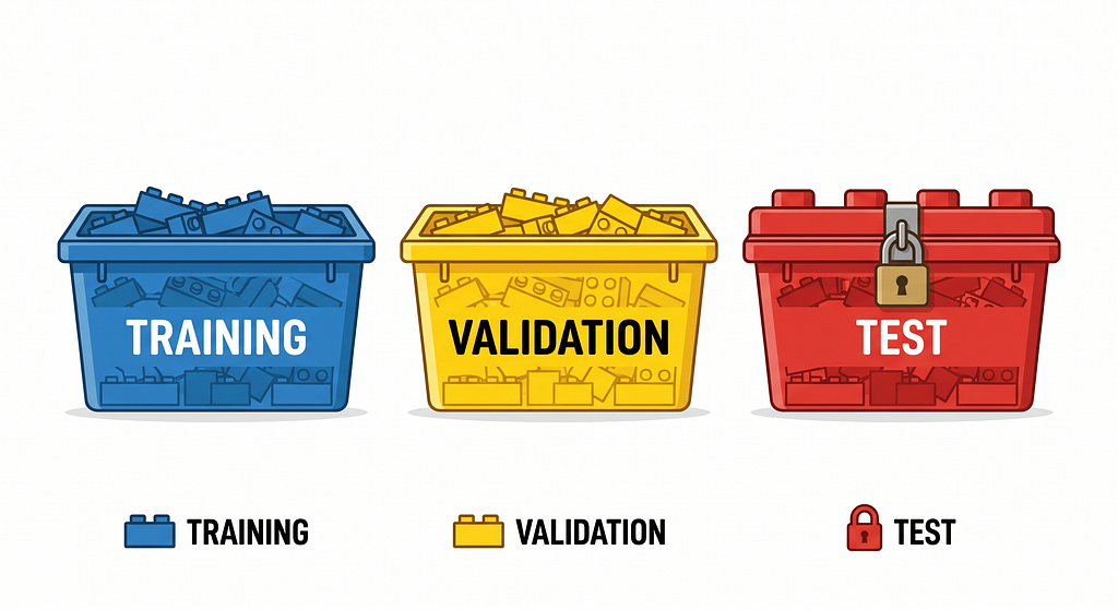
The standard approach is to split your data into three parts:

A training set (roughly 60–70%) that the model learns from.

A validation set(~15–20%) you use to tune and adjust it.

A test set (~15–20%) that stays locked away until the very end.

The test set is sacred. You don’t peek at it, use it to make decisions, or let it influence anything before final evaluation. It’s your one honest read on real-world performance.

The sneakier problem is data leakage — when information from the test world accidentally bleeds into training. It’s like giving students the exam the night before and then being surprised they score 100%. It happens in more ways than most people expect:

• You compute the average of your entire dataset before splitting, so the test data influences the normalization applied to training data
• A patient’s records appear in both training and test sets, so the model has effectively “seen” that patient
• You use a feature that encodes the answer — like “medication for diabetes” to predict “has diabetes”
• You use data that wouldn’t exist at prediction time, like next month’s sales to predict this month’s

When leakage happens, your model looks incredible in evaluation and fails immediately in production. It’s one of the most expensive mistakes in AI deployment, and it’s almost always invisible until it isn’t.

The fundamental tension every model faces

Here’s something that doesn’t get explained enough. Every model is trying to find the true pattern in data, and there are two ways to fail at that.

Draw a completely straight line through a scatter of curved dots: you’ve missed all the complexity. Your model is too simple — high bias, underfitting. It’s like a doctor who diagnoses everyone with the same disease regardless of symptoms.

Draw a wild squiggly line that passes through every single dot: you’ve memorized the noise rather than the pattern. Your model is too complex — high variance, overfitting. It’s like a student who memorizes every practice exam word-for-word and then fails the actual test because the questions are slightly different.

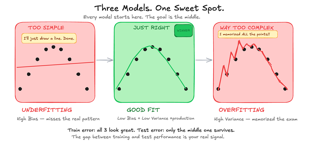
The sweet spot is a model that captures the real pattern without memorizing noise. And some noise simply cannot be removed — it’s the randomness of the world itself, irreducible.

The practical takeaway: if your model performs brilliantly on training data but poorly on validation, you’re overfitting. If it performs poorly on both, you’re underfitting. The gap between training and validation performance is your signal.

Using a single test split is often not enough

Here’s a subtle problem: what if you got lucky (or unlucky) with that particular split? Your evaluation score could vary significantly depending on which samples ended up in your test set.

K-Fold Cross-Validation fixes this. Instead of one split, you divide the data into k groups (folds). The model trains on k-1 folds and tests on the remaining one, then you rotate so every fold gets to be the test set once. Average the k scores. You get a much more reliable estimate with a measure of variance, not just a single number you got lucky with.

One hard rule for time series: never shuffle. You can’t train on future data to predict the past. The only valid approach is training on earlier time periods and testing on later ones — either with a fixed sliding window or an expanding window that grows over time.

The metrics that actually tell you something about classification

When your model predicts categories — spam or not spam, cancer or healthy, fraud or legitimate — accuracy is almost never the metric you should optimize for. Let me show you why.

If 99% of your transactions are legitimate and your model always predicts “legitimate,” it gets 99% accuracy. It catches zero fraud. Congratulations on your useless model.

Accuracy only means something when your classes are roughly balanced. For anything else, you need to understand where your model actually fails.

Start with the confusion matrix

The confusion matrix shows you exactly what’s going wrong. Every prediction your model makes falls into one of four buckets:

• True Positive (TP): model says fraud → it’s actually fraud ✓
• True Negative (TN): model says legitimate → it actually is legitimate ✓
• False Positive (FP): model says fraud → it was legitimate (blocked an innocent transaction)
• False Negative (FN): model says legitimate → it was fraud (let it through)

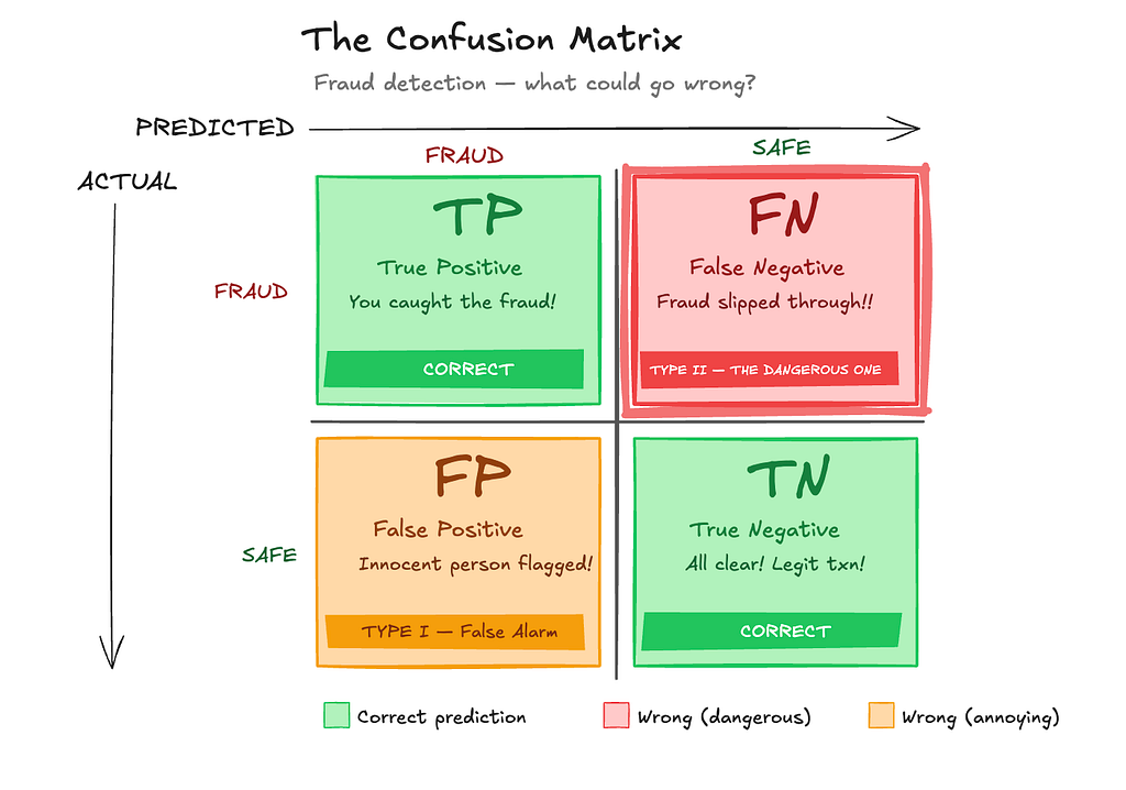
The matrix forces you to confront a question: which of these errors are you more afraid of?

An important point is this: positive does not mean good and negative does not mean bad. It just means the class we choose as the target event / class of interest. In fraud detection, that event is usually fraud, so fraud is treated as positive.

Precision and recall capture two different fears

Precision answers: of everything I flagged as positive, how many actually were?

Precision = TP / (TP + FP)

Think of a surgeon deciding whether to operate. If you operate on 10 patients and 9 of them didn’t need it, your precision is 10%. High precision means few false alarms.

Recall answers: of everything that was actually positive, how many did I catch?

Recall = TP / (TP + FN)

Think of a malaria screening test. If 100 people have malaria and you only catch 60, your recall is 60%. The 40 you missed were told they’re healthy and sent home. High recall means few misses.

These two metrics trade off against each other. Raise your detection threshold → you flag fewer things → what you do flag is more likely real (higher precision) but you miss more of the real cases (lower recall). There is no universally correct threshold. It depends entirely on what failure is more costly in your context.

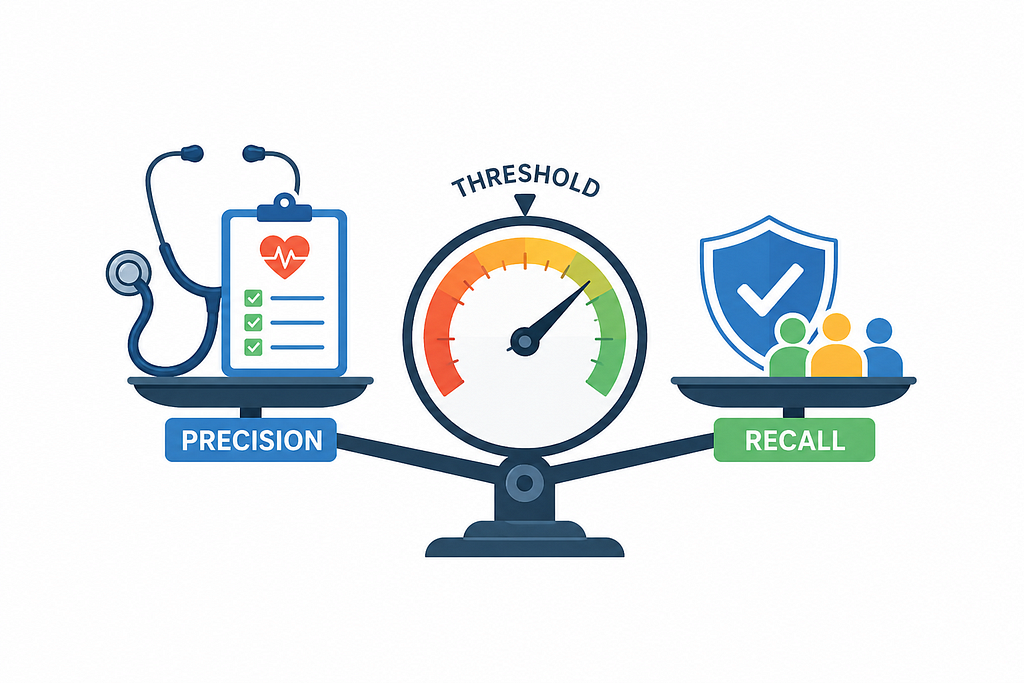
When both matter equally, use the F1 score — the harmonic mean of precision and recall. The harmonic mean matters here: if precision = 1.0 and recall = 0.0, F1 = 0, not 0.5. That’s the correct answer. A model that flags one thing and gets it right but misses everything else is a terrible model.

Two metrics that handle imbalance better than F1

Cohen’s Kappa corrects accuracy for the agreements you’d get by pure chance. Even random guessing agrees sometimes. Kappa asks: how much better than chance are you really?

The catch most people miss: a fraud model with 99% accuracy might have κ = 0.12 — “weak.” It’s just predicting “not fraud” for everything and getting lucky on the 99% that aren’t fraud.

MCC (Matthews Correlation Coefficient) is often the single most honest number for binary classification. Unlike F1, it considers all four cells of the confusion matrix equally. Unlike accuracy, it doesn’t collapse under class imbalance. The range is -1 to +1 (+1 = perfect, 0 = random, -1 = perfectly wrong). Use this when you want one number that doesn’t lie to you.

The ROC curve and AUC: the big picture

The ROC curve shows you the precision-recall tradeoff across every possible threshold at once. A random model sits on the diagonal. A perfect model jumps straight to the top-left corner (100% recall, zero false alarms). A real model lands somewhere in between, bowing toward the top-left.

AUC (Area Under the Curve) collapses this into one number. Here’s the clearest way to think about it: pick one real fraud and one real legitimate transaction at random. AUC is the probability that your model scores the fraud transaction higher. AUC = 0.85 means there’s an 85% chance it gets that right.

The cost of being wrong isn’t always symmetric

Not all errors cost the same, and optimizing for accuracy or F1 ignores that completely. A medical test that misses cancer is far worse than one that triggers a retest. A loan approval system that rejects a good client costs a different amount than one that approves a bad one.

The gain matrix forces you to put real numbers on it:

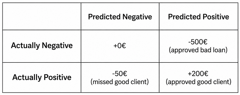
With this, your optimal threshold isn’t the one that maximizes accuracy — it’s the one that maximizes expected gain. This is how sophisticated financial and healthcare systems actually work, and it’s underused almost everywhere else.

Regression metrics: when the answer is a number

When your model predicts a continuous value — house prices, temperatures, energy consumption — you can’t use classification metrics. The four you need:

RMSE (Root Mean Squared Error) penalizes large errors heavily because of the squaring. A few badly wrong predictions dominate the score. If you’re predicting house prices and RMSE = €25,000, you’re typically off by about €25,000. Use this when big errors are especially costly.

MAE (Mean Absolute Error) treats all errors equally — no squaring. More robust when your data has outliers that would otherwise dominate RMSE.

R² tells you how much better your model is than just predicting the mean every time. R² = 1.0 is perfect. R² = 0.0 means you’re no better than “the average is always the answer.” R² < 0 means you’re actually worse than that, which is embarrassing.

MSE is just RMSE before you take the square root — useful mathematically but less intuitive since it’s in squared units.

Quick rule: outliers common → MAE. Large errors are especially bad → RMSE. Need to compare against a simple baseline → R².

The calibration problem nobody talks about enough

Most models don’t just predict a class — they output a probability. A fraud detector might say “87% chance this is fraud.” But does 87% actually mean fraud happens 87% of the time when the model says that? Often: no.

Calibration measures whether probability estimates match reality. Think of a weather app that says “70% chance of rain” on 100 different days. If it rains on exactly 70 of those days — perfect calibration. If it rains on only 40, the app is systematically overconfident.

The reliability diagram (plots predicted probability against observed fraction of positives in each probability bin) tells you the story visually. Perfect calibration lies on the diagonal. Curves below it indicate overconfidence, while curves above it indicate underconfidence.

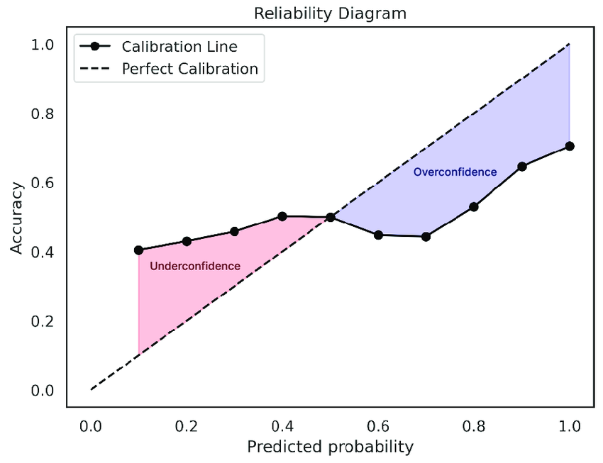
Why does this matter? If you’re using model scores to make decisions — fraud thresholds, medical risk scores, financial risk models — overconfident probabilities will systematically mislead you. You think you’re 90% certain. You’re not.

Expected Calibration Error (ECE) summarizes the average gap between predicted confidence and observed frequency across bins. An ECE of 0.05 means the model is off by about 5 percentage points on average across bins. Brier Score and Log-Loss evaluate probabilistic predictions more broadly. Both reward good probabilities and penalize confident mistakes, but Brier Score is not a pure calibration metric because it also reflects discrimination

If you find your model is miscalibrated, three post-training fixes: Platt Scaling (simple, works with little data), Isotonic Regression (flexible, needs more data), or Temperature Scaling (divide raw scores by a single parameter — elegant, widely used for neural networks).

Evaluating text, images, and code

For outputs beyond classifications and numbers, you need domain-specific metrics.

For text (translation, summarization, Q&A): the classic metrics count word overlap. BLEU favors precision — did the AI’s words appear in the reference? ROUGE favors recall — did the AI capture the key content from the reference? Both are fast and cheap, but they have a famous problem: “The cat sat on the mat” and “The feline was perched upon the rug” score as completely different sentences even though they mean the same thing.

BERTScore solves this by comparing meanings, not words — it converts both texts into embeddings and measures semantic similarity. Much more robust to paraphrasing.

For images (generative models): FID (Fréchet Inception Distance) compares the statistical distribution of generated images against real images — lower is more realistic and diverse. CLIP Score measures whether the generated image actually matches the text prompt you gave it.

For code: pass@k — generate k solutions, count it as a success if at least one passes all test cases. pass@1 is “one shot,” pass@10 is “one of ten tries.” This is fair because more attempts should give you a higher score.

For object detection: IoU (Intersection over Union) — what fraction of the combined bounding box area do the predicted and actual boxes share?

IoU ≥ 0.5 is the standard threshold for counting a detection as correct.

When humans have to be the judge

For a lot of AI outputs, there’s no clean automated metric. Is this chatbot response helpful? Does this essay flow? Is this image beautiful? You need human raters.

Before you put anyone in front of an evaluation interface, get clear on your rubric: what exactly are they rating, how should they score it, and what’s the difference between a 3 and a 4? Ambiguous rubrics produce noisy data that tells you nothing.

Inter-Annotator Agreement (IAA) tells you whether your rubric is working. If two raters agree on 60% of outputs, your task probably isn’t defined clearly enough. Cohen’s Kappa (for two raters) and Krippendorff’s Alpha (for many raters, different scales) are the standard measures.

The most powerful approach for LLM evaluation is pairwise comparison — not “rate this response 1–5” but “which of these two responses do you prefer?”

This is how modern LLMs are aligned: collect thousands of human preferences, train a reward model on them, use that to fine-tune the AI. It’s also how Chatbot Arena works — thousands of users compare two AI systems side-by-side without knowing which is which, votes become Elo ratings, and you get crowdsourced ground-truth rankings of AI systems that no benchmark can fake.

AI grading AI: LLM-as-a-Judge

Here’s an idea that seemed strange at first and is now everywhere: use a powerful language model to evaluate another model’s outputs.

It makes sense when you think about it. For open-ended generation — is this answer helpful? is the tone appropriate? is this factually accurate? — there’s often no clean automated metric. Hiring humans for every evaluation is slow and expensive. So you give a judge model the original prompt, the AI’s response, and a clear rubric. It outputs a score and reasoning.

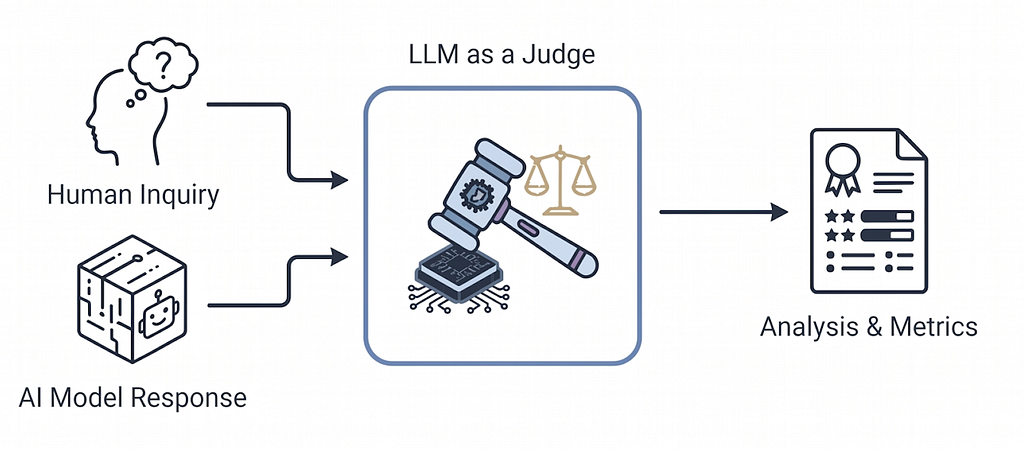
The caveats are real though. LLM judges have known biases:

— Position bias: they often prefer whichever response appears first

— Length bias: longer responses tend to score higher regardless of quality

— Self-serving bias: a model tends to rate its own outputs favorably

Mitigations: swap A/B positions and average, normalize for length, use a different model as judge than the one being evaluated, run multiple judge calls and average.

LLM-as-judge works well for helpfulness, tone, and factuality. For structured outputs (is this valid JSON?), use deterministic rules. For translation and summarization quality, start with BLEU/ROUGE then escalate to BERTScore when paraphrasing matters.

A tool we built for this: LevelApp

Running evaluations once before shipping is not evaluation — it’s theater. The real value comes from doing it continuously: before training, during development, before deployment, and after.

That’s why we built LevelApp — an evaluation framework for LLM-based applications. The frustration it was born from: every team we talked to was running evals in ad-hoc scripts, losing results, and not tracking how their AI system changed over time.

LevelApp is built around two ideas. The Simulator evaluates dialogue systems by simulating full conversations and scoring each reply with LLM-as-judge — you don’t have to manually run scripts. The Comparator evaluates structured outputs (extracted JSON, metadata) against ground truth.

pip install levelapp  # Python 3.12+

from levelapp.workflow import WorkflowConfig
from levelapp.core.session import EvaluationSession

config = WorkflowConfig.load(path="workflow_config.yaml")
with EvaluationSession(session_name="test", workflow_config=config) as session:
    session.run()
    results = session.workflow.collect_results()

It supports multiple evaluator types (LLM judge, reference-based, RAG-specific), multiple matching strategies (exact, fuzzy, semantic), multiple AI providers (OpenAI, Anthropic, Mistral, Gemini, Grok), and stores results in Firestore, filesystem, or MongoDB so you can track performance across versions over time.

The hard frontier: evaluating AI agents

Here’s where things get genuinely hard — and genuinely interesting.

Modern AI systems aren’t just models that answer one question. They’re agents: they use tools, make plans, browse the web, write and execute code, interact with databases, hand off work to other AI agents, and carry out multi-step tasks that unfold over minutes or hours. And evaluating them requires completely rethinking what “correct” means.

There are often many valid paths. If you ask an agent to “book a flight to Paris for under €500,” there might be dozens of valid solutions. Traditional evaluation asks “did you produce the right answer?” Agentic evaluation asks “did you accomplish the goal effectively?” These are very different questions.

Errors compound. A single bad decision early in a 20-step task can cascade into complete failure. A model that completes 18 of 20 steps correctly is vastly better than one that fails at step 3, but a simple pass/fail score treats them identically.

The process matters, not just the outcome. Did the agent use the minimum number of tool calls? Did it pick the right tool even when the wrong tool would have technically worked? Did it avoid unnecessary API calls that cost money or time?

Safety becomes a different kind of problem. An agent with file access, internet access, and code execution can cause real-world harm if it goes off the rails. Evaluating safety isn’t about one response — it’s about whether the agent ever takes a harmful action across a multi-hour task.

The field is using several approaches: task completion benchmarks(WebArena, SWE-bench, AgentBench) that define a goal state and check if the agent reached it; trajectory evaluation that scores each step, not just the final result; LLM-as-orchestrator-evaluator where a powerful model watches the agent’s full trace and evaluates its reasoning; and simulated environments where agents operate without real-world consequences.

The honest truth is we don’t have this solved. The open questions are live debates:

• What’s the unit of evaluation? One step? One task? One deployment?
• How do you handle non-determinism? The same agent can produce different results on the same task.
• How do you evaluate multi-agent systems where agents hand off work to each other?
• How do you prevent benchmark overfitting — teams optimizing for a benchmark until the benchmark stops measuring what it was meant to measure?

The most promising direction emerging is process reward models — instead of only rewarding the final answer, training models to evaluate intermediate reasoning steps. Whether that’s enough for complex agentic tasks, nobody knows yet.

What good evaluation actually looks like

Good evaluation is continuous, not a one-time checkpoint. The best teams evaluate at every stage:

Before training: understand your data distribution, actively hunt for leakage, set up your splits properly before you’ve ever looked at the test set.

During development: use cross-validation to get reliable estimates, compare models on the same held-out data, calibrate your probability outputs.

Before deployment: test on held-out data, run adversarial tests, check for safety issues, look at the errors specifically rather than just the average metric.

After deployment: monitor for metric drift (models degrade as the world changes), collect real user feedback, re-evaluate on new patterns that weren’t in the original test set.

The single most important shift is this: stop asking “what metric should I optimize?” and start asking “what failure mode am I most afraid of?” Then pick the metric that directly measures that. A fraud detection system with excellent Recall might block 30% of legitimate transactions and be undeployable. Excellent on paper. Useless in practice.

Metrics are proxies. Choose them carefully. Never stop checking.

Want to try LevelApp? pip install levelapp — full docs at pypi.org/project/levelapp

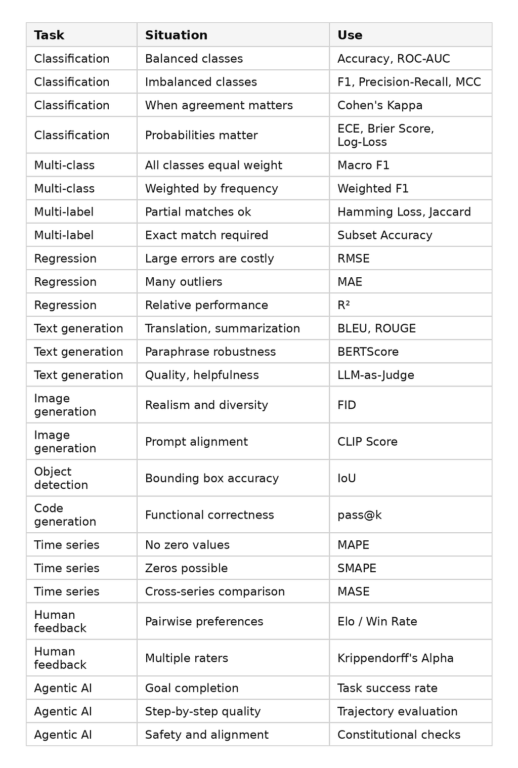
Quick reference: which metric when?